dir.create("data")
dir.create("output")Heatmaps in R
A worked example of making heatmaps in R with the ggplot2 package, as well as some data wrangling to easily format the data needed for the plot.
Learning objectives
- Manipulate data into a ‘tidy’ format
- Visualize data in a heatmap
- Become familiar with
ggplot2syntax for customizing plots
Heatmaps & data wrangling
Heatmaps are a great way of displaying three-dimensional data in only two dimensions. But how can we easily translate tabular data into a format for heatmap plotting? By taking advantage of “data munging” and graphics packages, heatmaps are relatively easy to produce in R.
Getting started
Workspace organization
First we need to setup our development environment. Open RStudio and create a new project via:
- File > New Project…
- Select ‘New Directory’
- For the Project Type select ‘New Project’
- For Directory name, call it something like “r-heatmaps” (without the quotes)
- For the subdirectory, select somewhere you will remember (like “My Documents” or “Desktop”)
Next create the two folders we’ll use to organize our efforts. The two folders should be data and output and will store…data and output.
For this lesson we will use data from a diversity survey of microbial life in a chrysotile asbestos mine. Driscoll and colleagues doi: 10.1016/j.gdata.2016.11.004 used next generation sequencing to identify and categorize bacterial diversity in a flooded pit of the abandoned mine. The data are normalized read counts for microbes found at the sites. A subset of the data can be downloaded from https://bit.ly/mine-data-csv (which itself redirects to https://raw.githubusercontent.com/jcoliver/learn-r/refs/heads/gh-pages/data/mine-micrsobe-class-data.csv). You can download this file to your computer with the download.file function:
download.file(url = "https://tinyurl.com/mine-data-csv",
              destfile = "data/mine-data.csv")
This downloads the data and saves it in the data directory as mine-data.csv.
Data Wrangling
We’ll need to start by reading the data into memory then formatting it for use by the ggplot package. We want all our work to be reproducible, so create a script where we can store all the commands we use to create the heatmap. We begin this script with brief information about the purpose of the script:
# Heatmap of mine pit microbe diversity
# Jeff Oliver
# jcoliver@email.arizona.edu
# 2017-06-05
Now we read those abundance data into memory:
mine_data <- read.csv(file = "data/mine-data.csv")Take a quick look at the structure of the data, using the str command:
str(mine_data)'data.frame': 8 obs. of 13 variables:
$ Site : int 1 2 3 1 2 3 2 3
$ Depth : num 0.5 0.5 0.5 3.5 3.5 3.5 25 25
$ Sample.name : chr "1-S" "2-S" "3-S" "1-M" ...
$ Actinobacteria : int 373871 332856 326695 409809 319778 445572 128251 96304
$ Cytophagia : int 8052 28561 10468 4481 15885 7302 4732 5566
$ Flavobacteriia : int 0 0 0 0 5230 6218 5917 6353
$ Sphingobacteriia : int 0 10013 4918 0 8274 8284 0 0
$ Nitrospira : int 0 0 0 0 0 0 4609 0
$ Planctomycetia : int 4553 10008 0 0 0 0 56836 67380
$ Alphaproteobacteria: int 143534 70575 105890 110746 52504 45000 133851 95580
$ Betaproteobacteria : int 124454 170161 187673 87245 146073 91711 90204 85707
$ Deltaproteobacteria: int 0 0 0 0 0 0 4260 0
$ Gammaproteobacteria: int 8426 9005 12935 7025 110825 69452 31956 165572The data frame has 8 rows (“obs.”) and 13 columns (“variables”). The first three columns have information about the observation (Site, Depth, Sample.name), and the remaining columns have the abundance for each of 10 classes of bacteria.
We ultimately want a heatmap where the different sites are shown along the x-axis, the classes of bacteria are shown along the y-axis, and the shading of the cell reflects the abundance. This latter value, the abundance of a bacteria at specific depths at different site, is really just a third dimension. However, instead of creating a 3-dimensional plot that can be difficult to visualize, we instead use shading for our “z-axis”. To this end, we need our data formatted so we have a column corresponding to each of these three dimensions:
- X: Sample identity
- Y: Bacterial class
- Z: Abundance
The challenge is that our data are not formatted like this. While the Sample.name column corresponds to what we would like for our x-axis, we do not have columns that correspond to what is needed for the y- and z-axes. All the data are in our data frame, but we need to take a table that looks like this:
| Site.name | Actinobacteria | Cytophagia |
|---|---|---|
| 1-S | 373871 | 8052 |
| 2-S | 332856 | 28561 |
| … | … | … |
And transform it to one with a column for bacterial class and a column for abundance, like this:
| Site.name | Class | Abundance |
|---|---|---|
| 1-S | Actinobacteria | 373871 |
| 1-S | Cytophagia | 8052 |
| 2-S | Actinobacteria | 332856 |
| 2-S | Cytophagia | 28561 |
| … | … | … |
Thankfully, there is an R package that does this for us! The tidyr package is designed for creating this type of “tidy”” data.
install.packages("tidyr")library("tidyr")In fact, we can do this transformation in one line with the pivot_longer function:
mine_long <- pivot_longer(data = mine_data,
                          cols = everything(),
                          names_to = "Class",
                          values_to = "Abundance")
Error in `pivot_longer()`:
! Can't combine `Site` <double> and `Sample.name` <character>.Uh oh. That error is preventing us from transforming our data to long format. What R is telling us is that we tried to create a column with multiple data types in it, which is a big no-no in R. That is, it attempted to make a single column that had both the data from the “Site” column (which are numbers) with the data from the “Sample.name” column, which is a factor (factors are what R calls categories).
Consider our original data structure:
str(mine_data)'data.frame': 8 obs. of 13 variables:
$ Site : int 1 2 3 1 2 3 2 3
$ Depth : num 0.5 0.5 0.5 3.5 3.5 3.5 25 25
$ Sample.name : chr "1-S" "2-S" "3-S" "1-M" ...
$ Actinobacteria : int 373871 332856 326695 409809 319778 445572 128251 96304
$ Cytophagia : int 8052 28561 10468 4481 15885 7302 4732 5566
$ Flavobacteriia : int 0 0 0 0 5230 6218 5917 6353
$ Sphingobacteriia : int 0 10013 4918 0 8274 8284 0 0
$ Nitrospira : int 0 0 0 0 0 0 4609 0
$ Planctomycetia : int 4553 10008 0 0 0 0 56836 67380
$ Alphaproteobacteria: int 143534 70575 105890 110746 52504 45000 133851 95580
$ Betaproteobacteria : int 124454 170161 187673 87245 146073 91711 90204 85707
$ Deltaproteobacteria: int 0 0 0 0 0 0 4260 0
$ Gammaproteobacteria: int 8426 9005 12935 7025 110825 69452 31956 165572Notice there are columns that don’t need to be transformed for our heatmap. Namely, Site, Depth, and Sample.name can all remain as-is. To do this, we instruct pivot_longer to ignore the first three columns of the data frame by negating those columns (-c(1:3):
mine_long <- pivot_longer(data = mine_data,
                          cols = -c(1:3),
                          names_to = "Class",
                          values_to = "Abundance")
head(mine_long)
# A tibble: 6 × 5
Site Depth Sample.name Class Abundance
<int> <dbl> <chr> <chr> <int>
1 1 0.5 1-S Actinobacteria 373871
2 1 0.5 1-S Cytophagia 8052
3 1 0.5 1-S Flavobacteriia 0
4 1 0.5 1-S Sphingobacteriia 0
5 1 0.5 1-S Nitrospira 0
6 1 0.5 1-S Planctomycetia 4553Another approach, to accomplish the same thing, especially if the columns to ignore are not adjacent, is to explicitly name the columns to ignore:
mine_long <- pivot_longer(data = mine_data,
                    cols = -c(Site, Depth, Sample.name),
                    names_to = "Class",
                    values_to = "Abundance")
To recap, at this point we read in the data and transformed it for easy use with heatmap tools:
# Heatmap of mine pit microbe diversity
# Jeff Oliver
# jcoliver@email.arizona.edu
# 2017-06-05

# Load dependancies
library("tidyr")

# Read data and format for heatmap
mine_data <- read.csv(file = "data/mine-data.csv")
mine_long <- pivot_longer(data = mine_data,
                    cols = -c(1:3),
                    names_to = "Class",
                    values_to = "Abundance")
Now the data are ready - on to the plot!
Plotting heatmaps
The ggplot package
To plot a heatmap, we are going to use the ggplot2 package.
install.packages("ggplot2")library("ggplot2")For this plot, we are going to first create the heatmap object with the ggplot function, then print the plot. We create the object by assigning the output of the ggplot call to the variable mine_heatmap, then entering the name of this object to print it to the screen.
mine_heatmap <- ggplot(data = mine_long, mapping = aes(x = Sample.name,
                                                       y = Class,
                                                       fill = Abundance)) +
  geom_tile() +
  xlab(label = "Sample")

mine_heatmap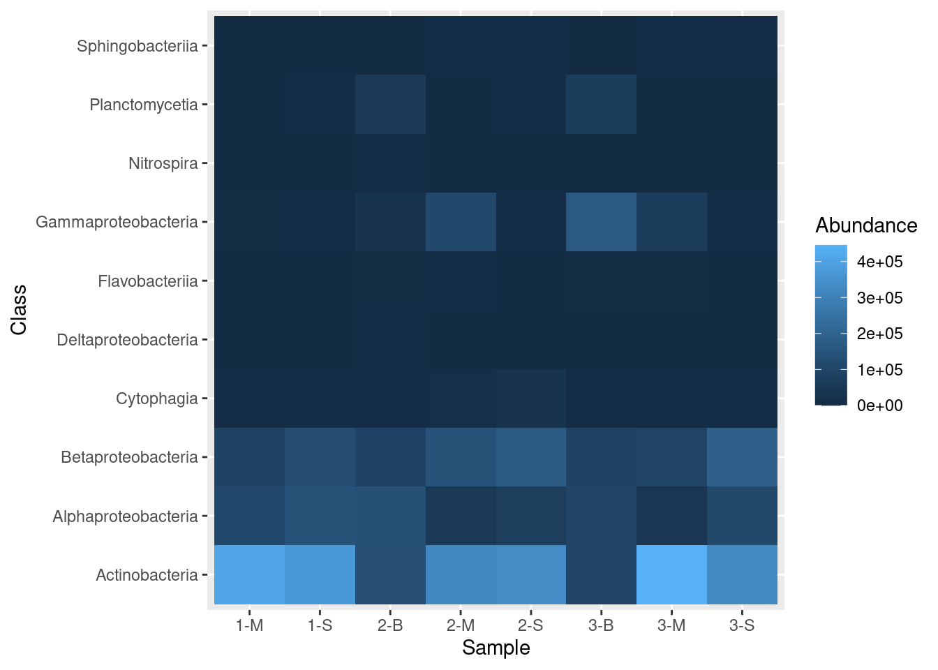
Let’s dissect these commands:
ggplotis the initial call, where we provide the following information:datais the data frame that contains the data we want to plotmappingtells ggplot what to plot where; that is, in this call, it says we want theSample.namecolumn on the x-axis, the bacterialClasson the y-axis, and the shading, or fill, (the z-axis) to reflect the value in theAbundancecolumn.
geom_tile, which is appended toggplotwith a plus sign (+), tells ggplot that we want a heatmapxlabprovides a label to use for the x-axis
This command follows the commonly used syntax for creating ggplot objects, where an initial call to ggplot sets up preliminary plotting information, and details are appended with plus signs:
# Create plot object
plot_object_name <- ggplot(data, mapping) +
  layer_one() +
  layer_two() +
  layer_three()

# Draw plot
plot_object_name
Faceting a plot
The ggplot package includes a great way to visualize different categories of data. This approach, called “faceting” requires one additional layer to the plotting command called facet_grid. With facet_grid we indicate which column contains the categories we want to use for the plot:
mine_heatmap <- ggplot(data = mine_long, mapping = aes(x = Sample.name,
                                                       y = Class,
                                                       fill = Abundance)) +
  geom_tile() +
  xlab(label = "Sample") +
  facet_grid(~ Depth)

mine_heatmap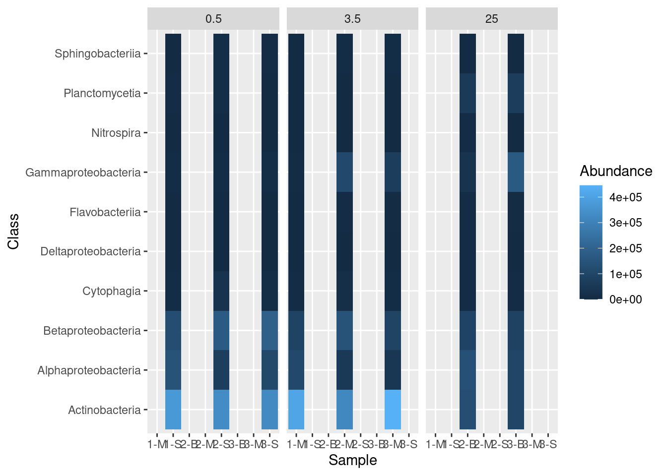
But this leaves a bit to be desired. We only want columns displayed for which there are data, so we have to add some additional information in our facet_grid call:
mine_heatmap <- ggplot(data = mine_long, mapping = aes(x = Sample.name,
                                                       y = Class,
                                                       fill = Abundance)) +
  geom_tile() +
  xlab(label = "Sample") +
  facet_grid(~ Depth, scales = "free_x", space = "free_x")

mine_heatmap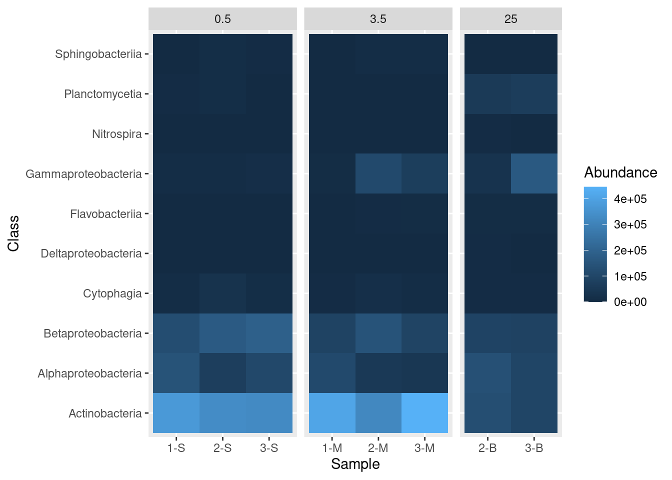
- Passing
"free_x"to thescalesargument instructs R to allow different x-axis for each of our sub-plots. In this case, the default is for each site to appear in each sub-plot. Specifyingscales = "free_x"removes any site from a sub-plot where there is no corresponding data. That is, it removes sites 1-S, 2-S, and 3-S from the 3.5 and 25 depth sub-plots, removes 1-M, 2-M, and 3-M from the 0.5 and 25 depth sub-plots, and removes 2-B and 3-B from the 0.5 and 3.5 depth sub-plots. - Passing
"free_x"tospaceensures that each column in the plot is the same width. Try it without specifying thespaceargument to see the effect of this behavior.
While we are here, we can also move the boxes labelling each sub-plot (0.5, 3.5, and 25) from the top of the plot to the bottom of the plot with the switch argument in the facet_grid() function:
mine_heatmap <- ggplot(data = mine_long, mapping = aes(x = Sample.name,
                                                       y = Class,
                                                       fill = Abundance)) +
  geom_tile() +
  xlab(label = "Sample") +
  facet_grid(~ Depth, switch = "x", scales = "free_x", space = "free_x")

mine_heatmap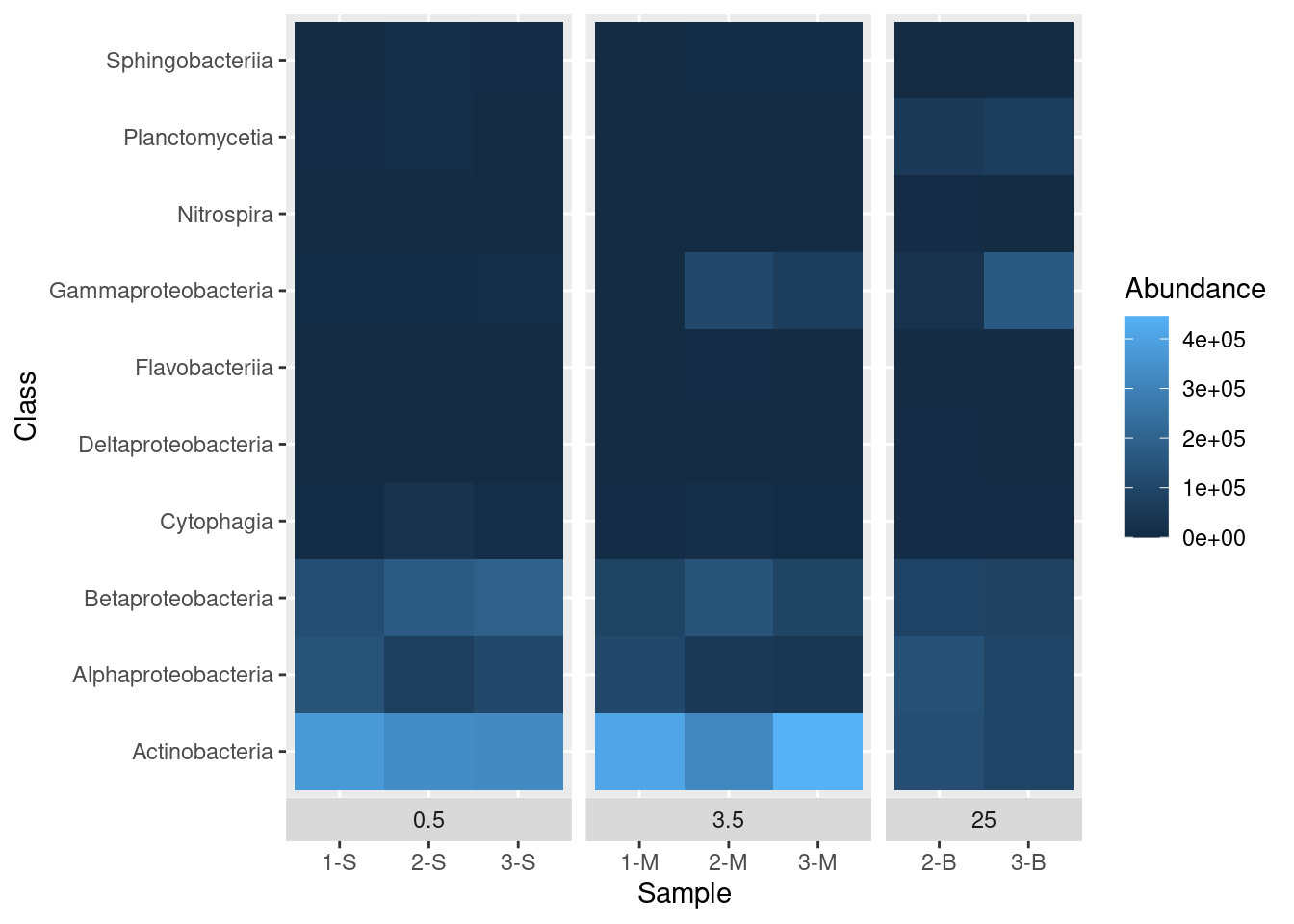
That’s better. There is still some room for improvement, but we’ll get to that later.
Improving aesthetics
Scale
First let’s deal with a scaling issue. Most values are dark blue, but this is partly caused by the distribution of values - there are a few really high values in the Abundance column. We can transform the data for display by taking the square root of abundance and plotting that. To do this, we need to add another column to our data frame and update our call to ggplot to reference this new column, Sqrt.abundance:
mine_long$Sqrt.abundance <- sqrt(mine_long$Abundance)
mine_heatmap <- ggplot(data = mine_long, mapping = aes(x = Sample.name,
                                                       y = Class,
                                                       fill = Sqrt.abundance)) +
  geom_tile() +
  xlab(label = "Sample") +
  facet_grid(~ Depth, switch = "x", scales = "free_x", space = "free_x")

mine_heatmap![]()
Color
What if we want to use a different set of colors besides the default? For example, how can we change the shading so low values are light and high values are dark? We change colours with scale_fill_gradient. In this case we pass three objects to scale_fill_gradient: name is a label to use in the legend and low and high are hex codes for color. In this case, we use white (#FFFFFF) for the low values and a dark blue (#012345) for high values.
mine_long$Sqrt.abundance <- sqrt(mine_long$Abundance)
mine_heatmap <- ggplot(data = mine_long, mapping = aes(x = Sample.name,
                                                       y = Class,
                                                       fill = Sqrt.abundance)) +
  geom_tile() +
  xlab(label = "Sample") +
  facet_grid(~ Depth, switch = "x", scales = "free_x", space = "free_x") +
  scale_fill_gradient(name = "Sqrt(Abundance)",
                      low = "#FFFFFF",
                      high = "#012345")

mine_heatmap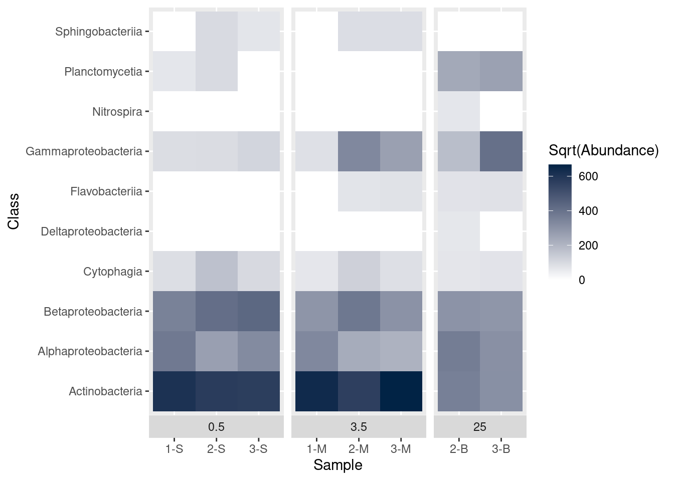
Theme elements
A number of elements of the plot are controlled through the theme function of ggplot. We can use this function to alter axis titles and the placement of the facet titles. Remember the facets? We grouped the graphs based on the depth of the samples. The graph currently shows the depth labels (the boxes with 0.5, 3.5, or 25) between the graph and the sample name. We’d like to swap these positions, so the categories are shown at the very bottom. While we’re at it, we should update the x-axis label, too. Setting strip.placement to “outside” should accomplish this.
mine_long$Sqrt.abundance <- sqrt(mine_long$Abundance)
mine_heatmap <- ggplot(data = mine_long, mapping = aes(x = Sample.name,
                                                       y = Class,
                                                       fill = Sqrt.abundance)) +
  geom_tile() +
  xlab(label = "Depth (m)") +
  facet_grid(~ Depth, switch = "x", scales = "free_x", space = "free_x") +
  scale_fill_gradient(name = "Sqrt(Abundance)",
                      low = "#FFFFFF",
                      high = "#012345") +
  theme(strip.placement = "outside")

mine_heatmap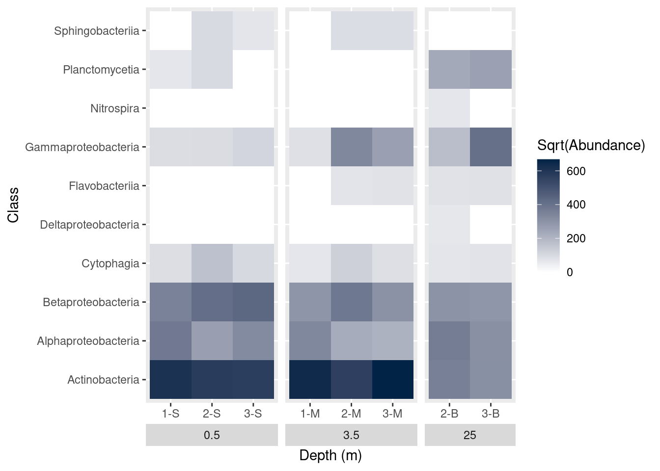
Plot title
Plot titles can be added with ggtitle:
mine_long$Sqrt.abundance <- sqrt(mine_long$Abundance)
mine_heatmap <- ggplot(data = mine_long, mapping = aes(x = Sample.name,
                                                       y = Class,
                                                       fill = Sqrt.abundance)) +
  geom_tile() +
  xlab(label = "Depth (m)") +
  facet_grid(~ Depth, switch = "x", scales = "free_x", space = "free_x") +
  scale_fill_gradient(name = "Sqrt(Abundance)",
                      low = "#FFFFFF",
                      high = "#012345") +
  theme(strip.placement = "outside") +
  ggtitle(label = "Microbe Class Abundance")

mine_heatmap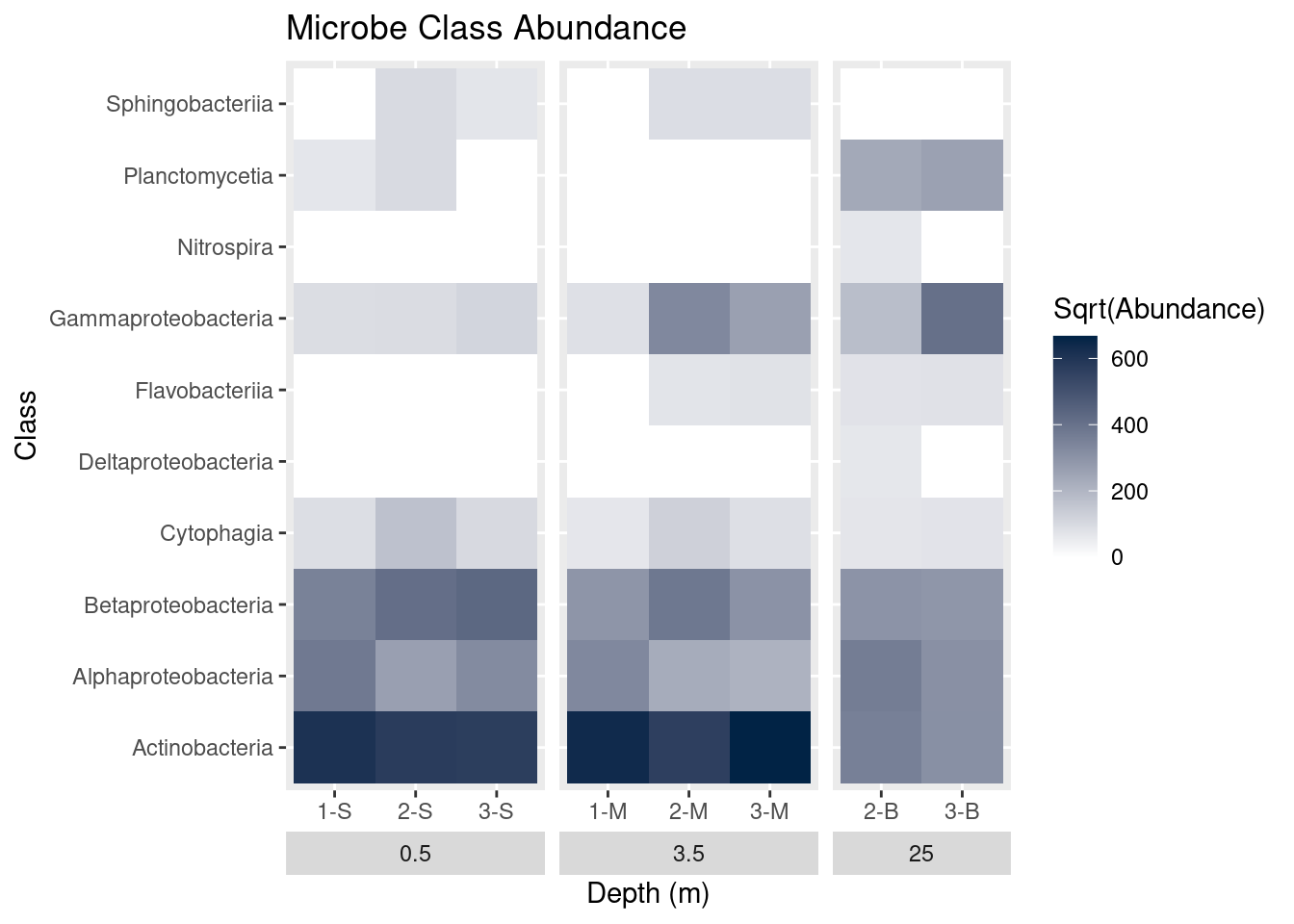
But by default the title is left-aligned. To center-justify the title, we add another argument, plot.title to the theme call:
mine_long$Sqrt.abundance <- sqrt(mine_long$Abundance)
mine_heatmap <- ggplot(data = mine_long, mapping = aes(x = Sample.name,
                                                       y = Class,
                                                       fill = Sqrt.abundance)) +
  geom_tile() +
  xlab(label = "Depth (m)") +
  facet_grid(~ Depth, switch = "x", scales = "free_x", space = "free_x") +
  scale_fill_gradient(name = "Sqrt(Abundance)",
                      low = "#FFFFFF",
                      high = "#012345") +
  theme(strip.placement = "outside",
        plot.title = element_text(hjust = 0.5)) +
  ggtitle(label = "Microbe Class Abundance")

mine_heatmap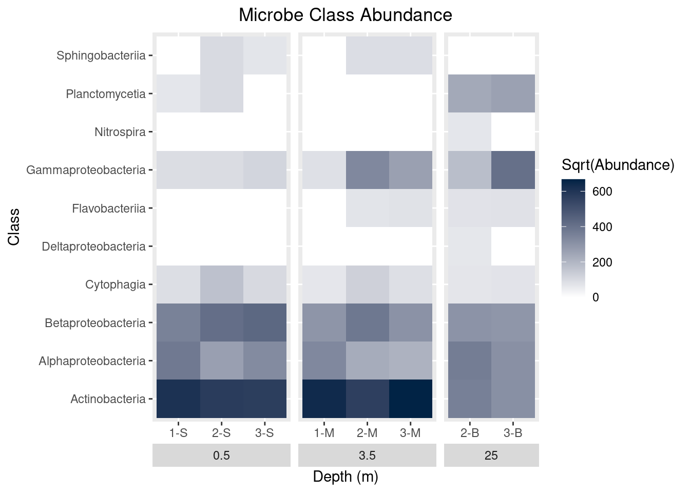
Miscellaneous Debris
There are a couple more things we will change in the plot:
- Reverse the order of the y-axis, so ‘Actinobacteria’ is at the top
- Remove the y-axis title
- Change the colors of the boxes for the depth categories
The second two are done via the theme command, with the axis.title.y and strip.background arguments. The first, though, requires consideration of how ggplot determines the order of the y-axis. When the axis values are categories, ggplot treats them as factors and places them, from bottom to top, in the order of the levels for the factor. Since we are using values in the Class column, take a look at the default order if the column is treated as a factor:
levels(as.factor(mine_long$Class)) [1] "Actinobacteria" "Alphaproteobacteria" "Betaproteobacteria"
[4] "Cytophagia" "Deltaproteobacteria" "Flavobacteriia"
[7] "Gammaproteobacteria" "Nitrospira" "Planctomycetia"
[10] "Sphingobacteriia" Since Actinobacteria is the first level, it appears at the bottom of the y-axis; the last level is Sphingobacteriia and appears at the top of the plot. To reverse this order, we use scale_y_discrete and pass the factor levels in reverse. What? Take another look at the output of the levels command. If we wanted to reverse this output, we can use the rev function:
rev(levels(as.factor(mine_long$Class))) [1] "Sphingobacteriia" "Planctomycetia" "Nitrospira"
[4] "Gammaproteobacteria" "Flavobacteriia" "Deltaproteobacteria"
[7] "Cytophagia" "Betaproteobacteria" "Alphaproteobacteria"
[10] "Actinobacteria" Now we use the same command in scale_y_discrete for the limits argument:
mine_long$Sqrt.abundance <- sqrt(mine_long$Abundance)
mine_heatmap <- ggplot(data = mine_long, mapping = aes(x = Sample.name,
                                                       y = Class,
                                                       fill = Sqrt.abundance)) +
  geom_tile() +
  xlab(label = "Depth (m)") +
  facet_grid(~ Depth, switch = "x", scales = "free_x", space = "free_x") +
  scale_fill_gradient(name = "Sqrt(Abundance)",
                      low = "#FFFFFF",
                      high = "#012345") +
  theme(strip.placement = "outside",
        plot.title = element_text(hjust = 0.5)) +
  ggtitle(label = "Microbe Class Abundance") +
  scale_y_discrete(limits = rev(levels(as.factor(mine_long$Class))))

mine_heatmap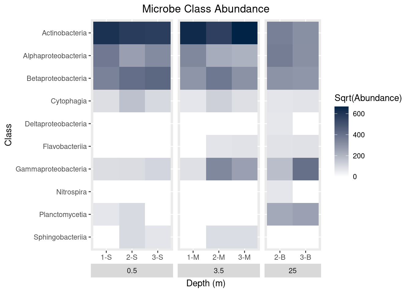
And to adjust the y-axis and change the depth boxes, we add two more arguments to the theme command:
mine_long$Sqrt.abundance <- sqrt(mine_long$Abundance)
mine_heatmap <- ggplot(data = mine_long, mapping = aes(x = Sample.name,
                                                       y = Class,
                                                       fill = Sqrt.abundance)) +
  geom_tile() +
  xlab(label = "Depth (m)") +
  facet_grid(~ Depth, switch = "x", scales = "free_x", space = "free_x") +
  scale_fill_gradient(name = "Sqrt(Abundance)",
                      low = "#FFFFFF",
                      high = "#012345") +
  theme(strip.placement = "outside",
        plot.title = element_text(hjust = 0.5),
        axis.title.y = element_blank(), # Remove y-axis title
        strip.background = element_rect(fill = "#EEEEEE", color = "#FFFFFF")) +
  ggtitle(label = "Microbe Class Abundance") +
  scale_y_discrete(limits = rev(levels(as.factor(mine_long$Class))))

mine_heatmap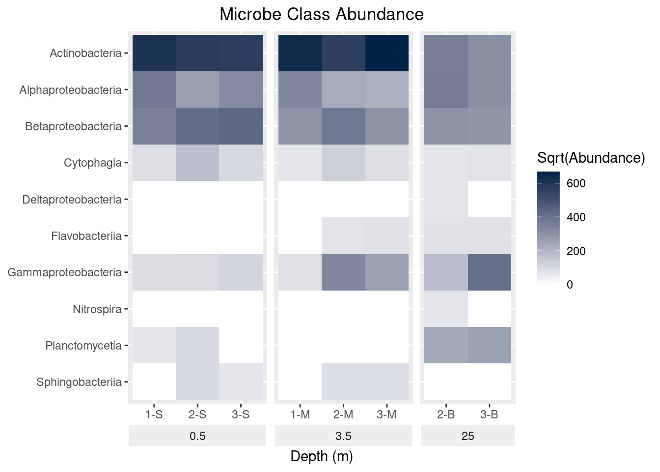
Finally, there are many default themes in ggplot that affect background colors, grid lines, and fonts. You can see examples of them in use at https://ggplot2.tidyverse.org/reference/ggtheme.html. One relatively simple theme is theme_bw, and we can apply it by adding the function to our ggplot object:
mine_long$Sqrt.abundance <- sqrt(mine_long$Abundance)
mine_heatmap <- ggplot(data = mine_long, mapping = aes(x = Sample.name,
                                                       y = Class,
                                                       fill = Sqrt.abundance)) +
  geom_tile() +
  xlab(label = "Depth (m)") +
  facet_grid(~ Depth, switch = "x", scales = "free_x", space = "free_x") +
  scale_fill_gradient(name = "Sqrt(Abundance)",
                      low = "#FFFFFF",
                      high = "#012345") +
  theme(strip.placement = "outside",
        plot.title = element_text(hjust = 0.5),
        axis.title.y = element_blank(),
        strip.background = element_rect(fill = "#EEEEEE", color = "#FFFFFF")) +
  ggtitle(label = "Microbe Class Abundance") +
  scale_y_discrete(limits = rev(levels(as.factor(mine_long$Class)))) +
  theme_bw() # Use the black and white theme

mine_heatmap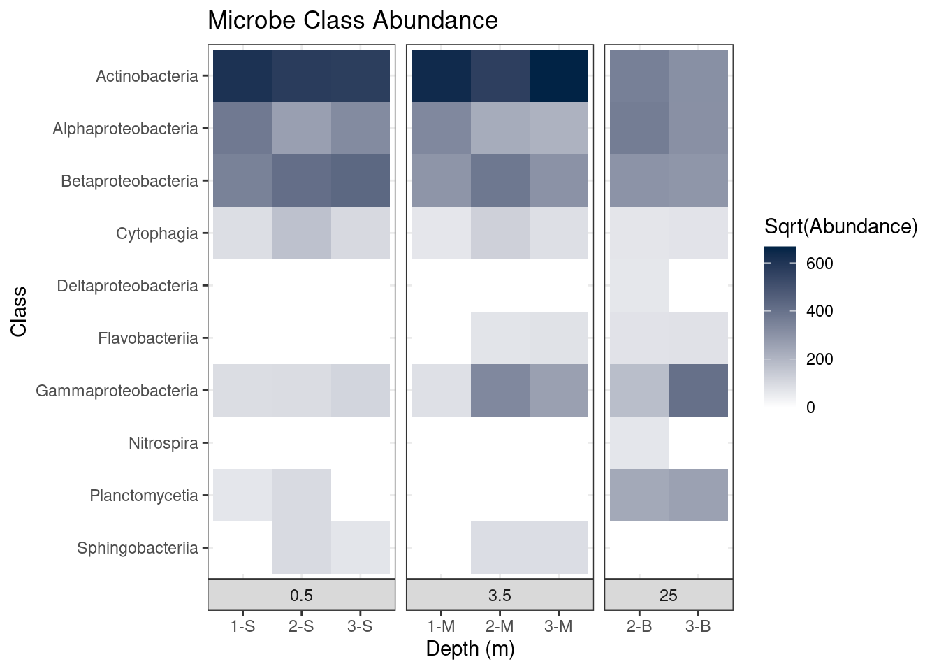
Most notably, the different depth plots all have a black border around them. But if we take a closer look, a number of our changes have been undone! The shading of the boxes indicating Depth is darker, the labels for the samples are back at the bottom, and the y-axis title (“Class”) has returned.
Why did this happen? Didn’t we fix all of that with the call to theme?
This demonstrates the importance of order in building ggplot objects. When we use the function theme_bw, we are using the settings in theme_bw for all theme elements. Thus by adding theme_bw after our call to theme, we effectively throw out all those changes we made. In order for our changes to stay in place, we will need to call theme_bw before our call to theme:
mine_long$Sqrt.abundance <- sqrt(mine_long$Abundance)
mine_heatmap <- ggplot(data = mine_long, mapping = aes(x = Sample.name,
                                                       y = Class,
                                                       fill = Sqrt.abundance)) +
  geom_tile() +
  xlab(label = "Depth (m)") +
  facet_grid(~ Depth, switch = "x", scales = "free_x", space = "free_x") +
  scale_fill_gradient(name = "Sqrt(Abundance)",
                      low = "#FFFFFF",
                      high = "#012345") +
  theme_bw() +
  theme(strip.placement = "outside",
        plot.title = element_text(hjust = 0.5),
        axis.title.y = element_blank(),
        strip.background = element_rect(fill = "#EEEEEE", color = "#FFFFFF")) +
  ggtitle(label = "Microbe Class Abundance") +
  scale_y_discrete(limits = rev(levels(as.factor(mine_long$Class))))

mine_heatmap
Our final script for this heatmap is then:
# Heatmap of mine pit microbe diversity
# Jeff Oliver
# jcoliver@email.arizona.edu
# 2017-06-05

# Load dependancies
library("tidyr")
library("ggplot2")

# Read data and format for heatmap
mine_data <- read.csv(file = "data/mine-data.csv")
mine_long <- pivot_wider(data = mine_data,
                         cols = -c(1:3),
                         names_to = "Class",
                         values_to = "Abundance")

# Transform abundance data for better visualization
mine_long$Sqrt.abundance <- sqrt(mine_long$Abundance)

# Plot abundance
mine_heatmap <- ggplot(data = mine_long, mapping = aes(x = Sample.name,
                                                       y = Class,
                                                       fill = Sqrt.abundance)) +
  geom_tile() +
  xlab(label = "Depth (m)") +
  # Facet on depth and drop empty columns
  facet_grid(~ Depth, switch = "x", scales = "free_x", space = "free_x") +
  # Set colors different from default
  scale_fill_gradient(name = "Sqrt(Abundance)",
                      low = "#FFFFFF",
                      high = "#012345") +
  theme_bw() +

  theme(strip.placement = "outside", # Move depth boxes to bottom of plot
        plot.title = element_text(hjust = 0.5), # Center-justify plot title
        axis.title.y = element_blank(), # Remove y-axis title
        strip.background = element_rect(fill = "#EEEEEE", color = "#FFFFFF")) +
  ggtitle(label = "Microbe Class Abundance") +
  scale_y_discrete(limits = rev(levels(as.factor(mine_long$Class))))

mine_heatmap
Additional resources
- Paper describing tidy data
- A great introduction to data tidying
- A cheat sheet for data wrangling
- Official documentation for ggplot
- A cheat sheet for ggplot
- Documentation for
geom_bin2d, to create heatmaps for continuous x- and y-axes - A PDF version of this lesson